Learn How To Graph Absolute Value Functions

This video describes absolute value functions and how they are graphed. After you finish this lesson, view all of our Algebra 1 lessons and practice problems.

Absolute value functions are similar to regular linear functions, except the absolute value of the bracketed items can never be negative. The absolute value of any number is the measure of its distance from 0, so the graph for an absolute value function will appear shaped like a “V”.

A translation is a shift of a function on the coordinate plane. An absolute value function can be shifted vertically and horizontally.

If a constant is added/subtracted outside of the absolute value bars (ex. $|x|+1$ ), the function shifts up or down the amount of units indicated (‘+’ = up, ‘-‘ = down)

If a constant is added/subtracted within the absolute value bars ( $|x+1|$ ), the function shifts left or right the amount of units indicated. (*** ‘+’ = shift to the LEFT, ‘-‘ shift to the RIGHT***)

An absolute value function can also be dilated or compressed.

If a function is multiplied by a constant larger than one ( $2|x|$ ), the absolute value function COMPRESSES (narrower).

If a function is multiplied by a constant smaller than one ( $\frac{1}{2}|x|$ ), the absolute value function STRETCHES (wider).

Graphing can be done by creating a table and plugging in values to find coordinates.

Video-Lesson Transcript

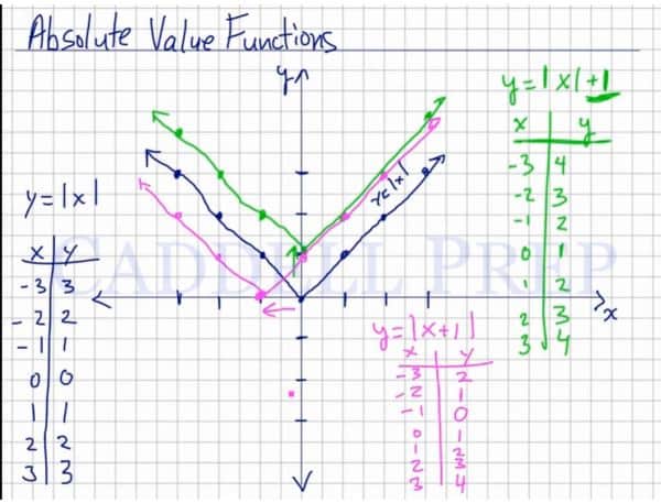
Let’s go over graphing absolute value functions.

So the actual basic line is $y = \mid x \mid$

So if $x = -3$ then $y = 3$ ,

$x = -2$ then $y = 2$ ,

$x = -1$ then $y = 1$ ,

$x = 0$ then $y = 0$ ,

$x = 1$ then $y = 1$ ,

$x = 2$ then $y = 2$ ,

and $x = 3$ then $y = 3$ .

Now let’s graph this using the coordinates above.

Our line looks like the letter “V”.

Let’s have a more complicated one.

For example:

$y = \mid x \mid + 1$

Let’s get the value of $x$ and $y$ .

If $x = -3$ then $y = 4$ ,

$x = -2$ then $y = 3$ ,

$x = -1$ then $y = 2$ ,

$x = 0$ then $y = 1$ ,

$x = 1$ then $y = 2$ ,

$x = 2$ then $y = 3$ ,

and $x = 3$ then $y = 4$ .

If we graph this, we’ll have another line that looks like a letter “V”.

But since we added $1$ to the absolute value of $x$ , we shifted the whole function up by $1$ spot.

Let’s have another example.

$y = \mid x + 1 \mid$

Let’s get the value of $x$ and $y$ .

If $x = -3$ then $y = 2$ ,
$x = -2$ then $y = 1$ ,
$x = -1$ then $y = 0$ ,
$x = 0$ then $y = 1$ ,
$x = 1$ then $y = 2$ ,
$x = 2$ then $y = 3$ ,
and $x = 3$ then $y = 4$ .

Let’s graph this now.

It looks the same but the function line moved towards the left by $1$ spot as compared with our first example.

So, if we’re going to add a number after we get the absolute value of $x$ , we’re going to move up.

And if we add a number to the value of $x$ before you get the absolute value, we’ll move to the left.

Here’s a more graphic representation:

$y = \mid x \mid + \#$ then we move up by that number;

if $y = \mid x \mid - \#$ then we’re going down by that number;

then if $y = \mid x + \# \mid$ then we’re going to the left by that number;

and if $y = \mid x - \# \mid$ then we’ll move to the right by that number.

For example, we have $y = \mid x - 5 \mid$ , then we’re going to move to the right by $5$ spots.

Let’s look at these two examples:

$y = \mid x + 3 \mid + 4$

$y = \mid x - 5 \mid - 2$

Let’s draw the regular absolute value graph as our base graph.

To draw the examples, let’s apply the rules above.

So in $y = \mid x + 3 \mid + 4$ , we will move $3$ spots to the left and up by $4$ .

Now, in $y = \mid x - 5 \mid - 2$ , we’re going to move to the right $5$ spots and down by $2$ spots.

Again, we’ll start with the absolute value graph.

For example, we have

$y = 2 \mid x \mid$

we will multiply the absolute value by a constant number that’s greater than $1$ .

Instead of our regular slope, we’ll have a slope steeper by that number. In our example, it’s $2$ spots.

Let’s have $y = 4 \mid x \mid$

We’ll have a line that the slope is up by $4$ spots.

Let’s see what happens if we multiply the absolute value by a fraction.

$y = \dfrac{1}{2} \mid x \mid$

Then, we’ll have a line that’s less steep.

The line will be wider than the regular one.

Next, let’s see what happens when the absolute value has a negative in front.

$y = - \mid x \mid$

Here, our line will be upside down as compared to the regular absolute value function.

Let’s have $y = -3 \mid x \mid$

We’ll have a line that goes down by $3$ spots.

Let’s have another example.

$y = - \mid x + 1 \mid + 2$

Here, it’s negative so our line will be upside down, $+ 1$ so we’ll move to the left by $1$ , and $+ 2$ so we’ll go up by $2$ .