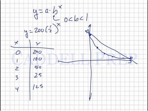
Learn About The Properties Of Exponential Decay And Its Functions

In this video, we are going to look at exponential decay. After you finish this lesson, view all of our Algebra 1 lessons and practice problems.

$y=a \times (b)^x$
For a graph to demonstrate exponential decay, the base of the exponent, b, must be between 0 and 1. These graphs decrease by a factor, and will not fall into the negatives.
For example:
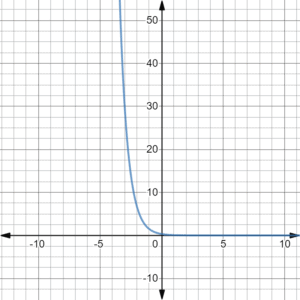
The graph of
$y=200 \times (\frac{1}{2})^x$
curves slowly downward after plotting points as shown in the video, and demonstrates exponential decay. This graph decreases by a factor of $\frac{1}{2}$ .

Examples of Exponential Decay

Example 1

Does the function $f=\dfrac{1}{3}\cdot \left(\dfrac{2}{9}\right)^x$ model exponential decay?

Yes, it shows an exponential decay since the value of $b$ is less than $1$ and the curve is slowly downward.

Example 2

What is the shape of the graph of the function $y=0.32(0.5^x)$ ?
Now, let’s solve for y and plot the coordinates

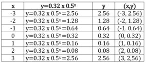
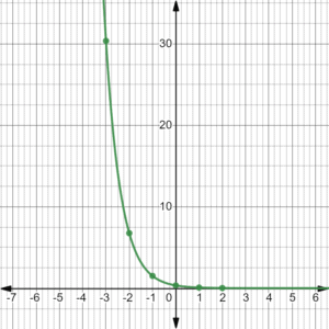
The graph shows a decreasing function. This is an exponential decay.

Video-Lesson Transcript

Let’s go over exponential decay.

Exponential decay is when something decreases by a certain factor over and over again.

You may see this in a chemistry problem or something like that nature.

For example:

We have $200$ g of something. It decreases half of the amount so now we have $100$ g. Then decrease by half again, we have $50$ g. Then decrease by half again, we have $25$ g. Then decrease by half again, so we have $12.5$ g. And so on.

Here, it decreases by a factor.

It is very different with a linear decay.

Where we have $200$ g and when we decrease it by $100$ g, we’ll have $100$ g. And if we decrease it by $100$ g again, we’ll have $0$ .

Or let’s decrease at $25$ g.

So we have $200$ g then decrease to $175$ . Then decrease again by $25$ , we’ll have $150$ .
And so on.

In exponential decay, we keep decreasing and the amount we decrease by also keeps on decreasing.

Whereas in a linear decay, it keeps on decreasing by a certain amount over and over again.

If we think about the linear exponential function we have

$y = ab^x$

In exponential decay, $0 \textless b \textless 1$ . So its somewhere between $0$ and $1$ .

For example:

$y = 200 (\dfrac{1}{2})^x$

This one models the one we have before. Whereas $200$ decreases by $\dfrac{1}{2}$ over and over again.

So initially, at time $0$ , we have $200$ .

When $x = 1$ then $y = 100$ ,
$x = 2$ then $y = 50$ ,
$x = 3$ then $y = 25$ ,
$x = 4$ then $y = 12.5$ ,
and so on.

Let’s graph this.

But if we have a linear decrease, we’ll have a straight line decrease.

The exponential decay line will not pass through the $x$ axis.

Whereas, the linear decay line will go down into the negatives.